Step 1: Start the Graphical User Interface
After installing pyMolDyn, use
% pymoldyn
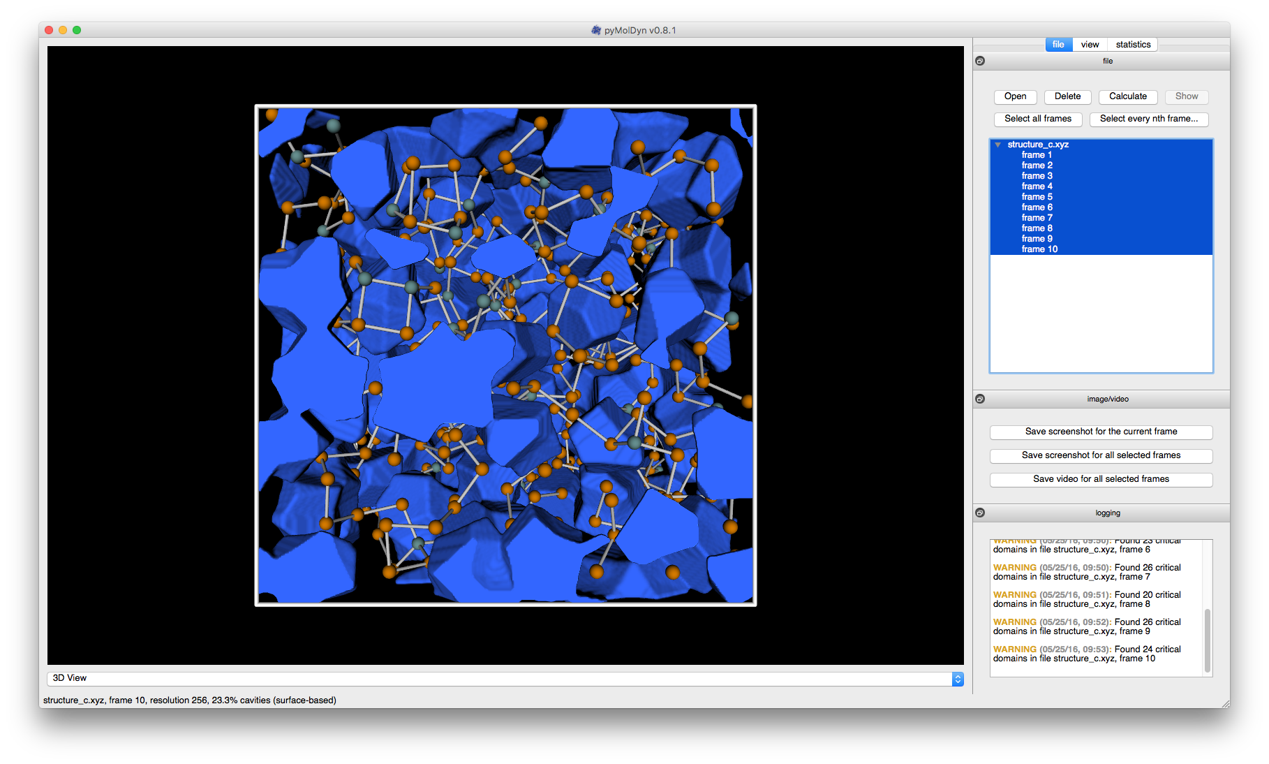
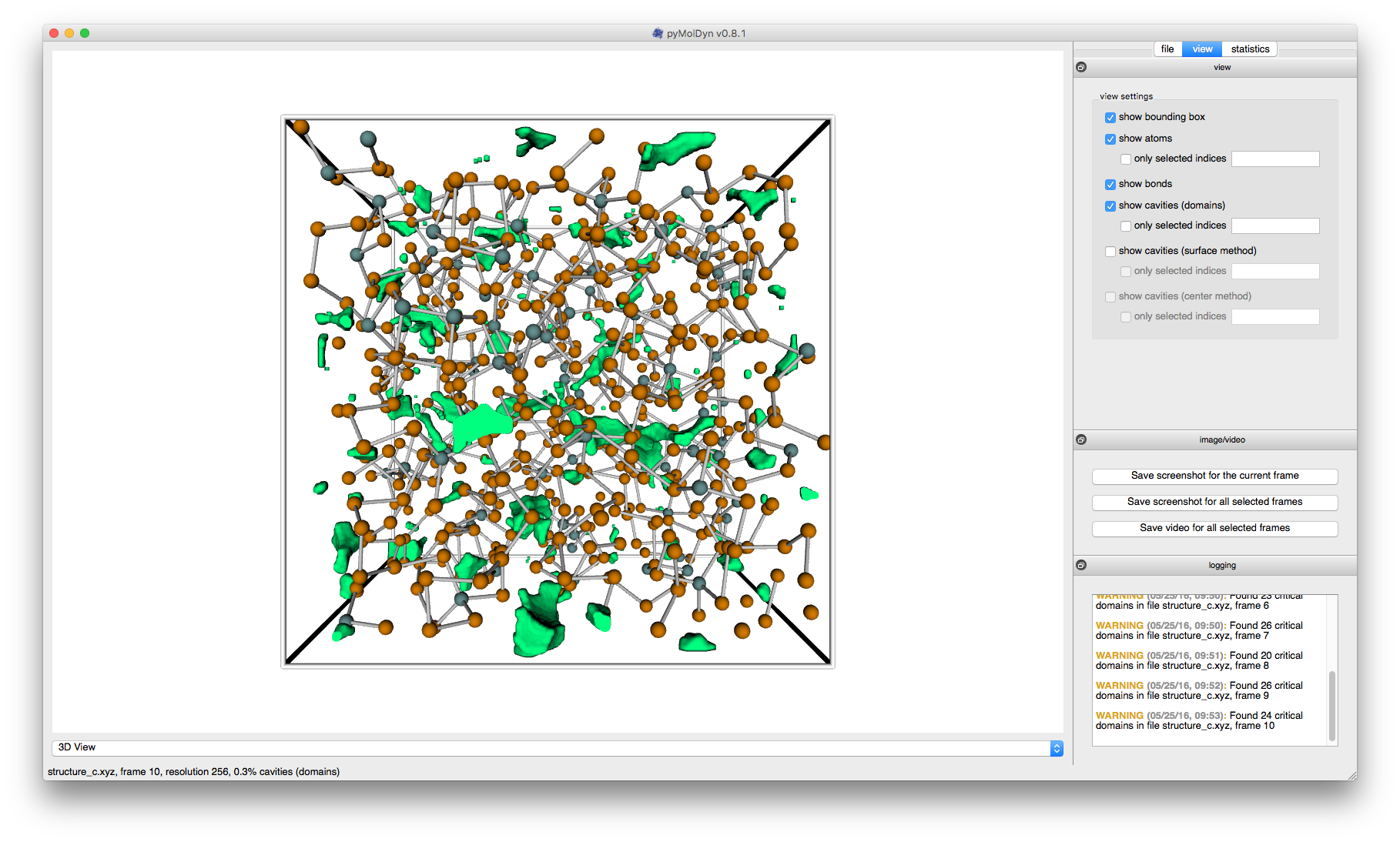
to launch the GUI. The window pictured below will open.
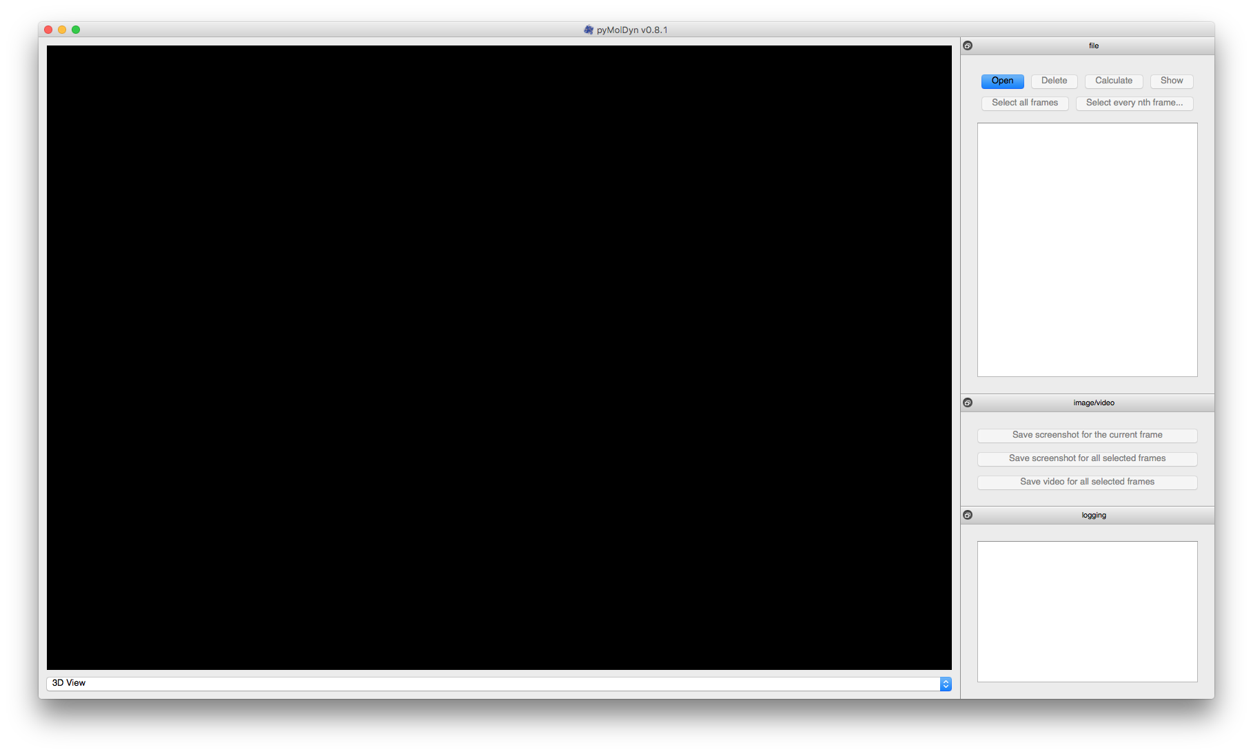
The black area is where atoms, bonds and cavities will be displayed. The bar underneath (3D view, Pair distribution functions, Cavity Histograms) provides access to further information (see below). The area on the right consists of three tabs:
- file: for opening files and starting calculations
- view: for controlling what is shown on the left side
- statistics: for information on the atoms and cavities in the currently opened frame
The statistics tab is hidden until you first open a frame.
In addition to these tabs, the image/video panel for exporting screenshots or videos and a logging window for calculation warnings are placed at the bottom right of the window.
Step 2: Loading an XYZ file
In the file tab, click Open. This will open a file selection dialog. Select the file you want to use and confirm
this selection by clicking Open in the dialog. Please ensure, that the comment line in your XYZ file includes a
description of its cell, e.g. CUB 27.5 for a cubic cell with a side length of 27.5Å. The file will be read and
inserted into the list in the file tab.
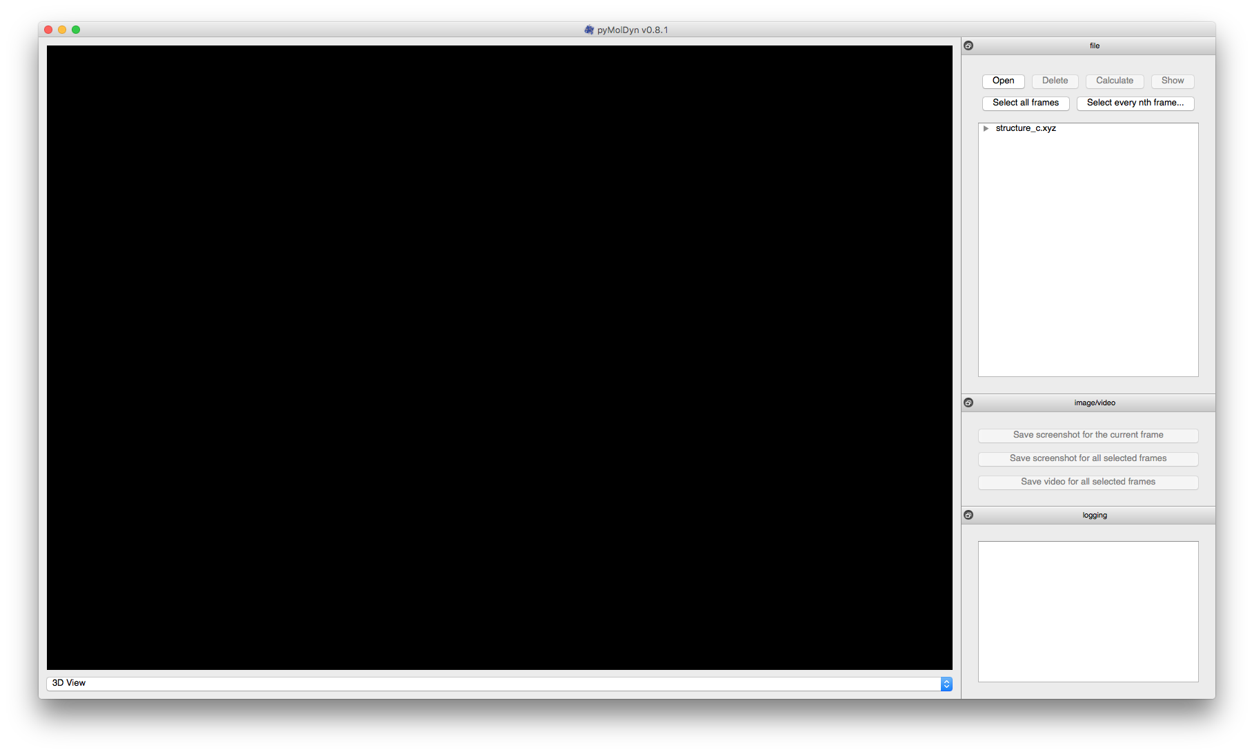
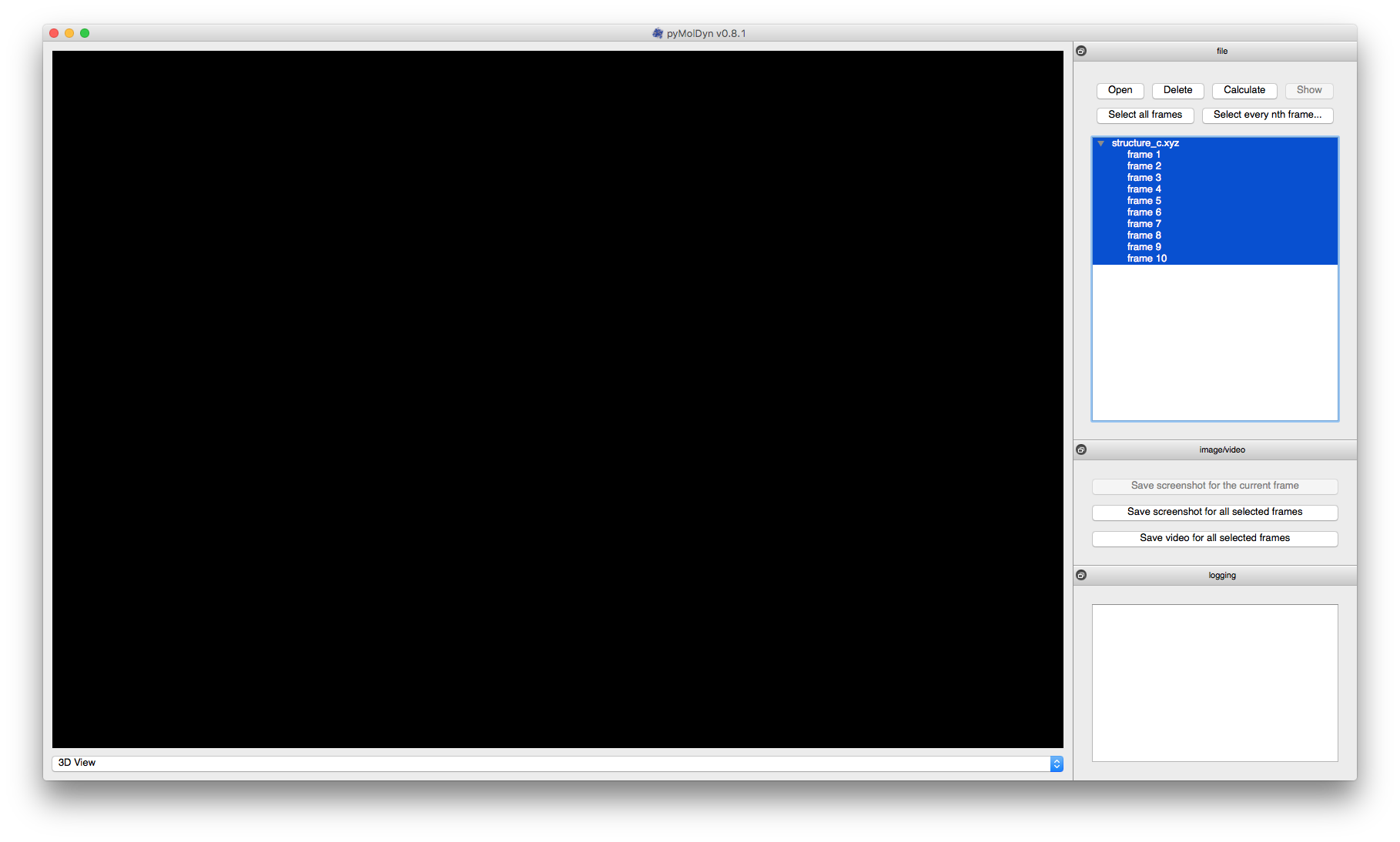
You can click on the small triangle symbol next to the file name to show a list of the frames in this file.
Step 3: Calculating Cavities
After selecting the frames for which cavities are to be calculated (e.g., by clicking on the file name to select all corresponding frames), click on the Calculate button.
The Calculation Settings dialog allows setting the resolution of the discretization used during the calculation, shows previous calculations performed for this dataset and offers further customizations. Results can be exported as text (ASCII) or HDF5 files. Alternatively, you can export selected data (text only) using the application menu (File → Export) or using keyboard shortcuts.
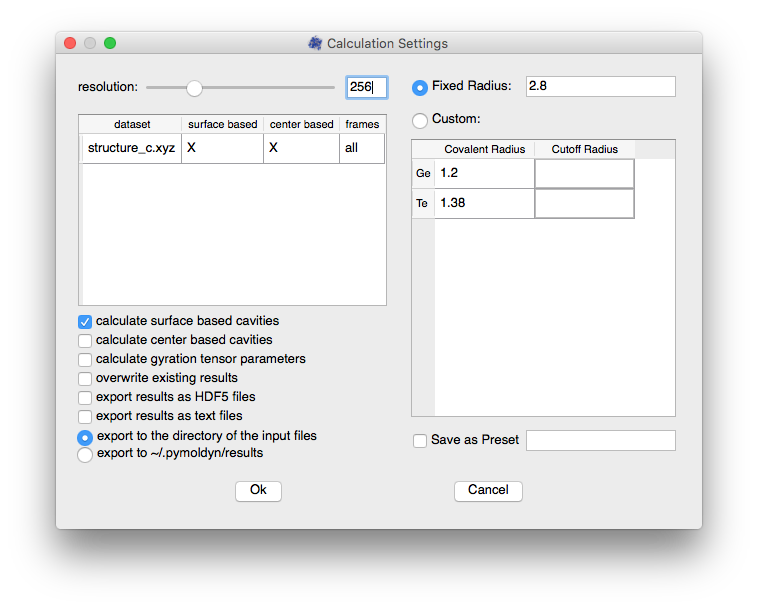
To start the calculation, click Ok. This will cause a progress dialog to open and, once the calulations are done, close again.
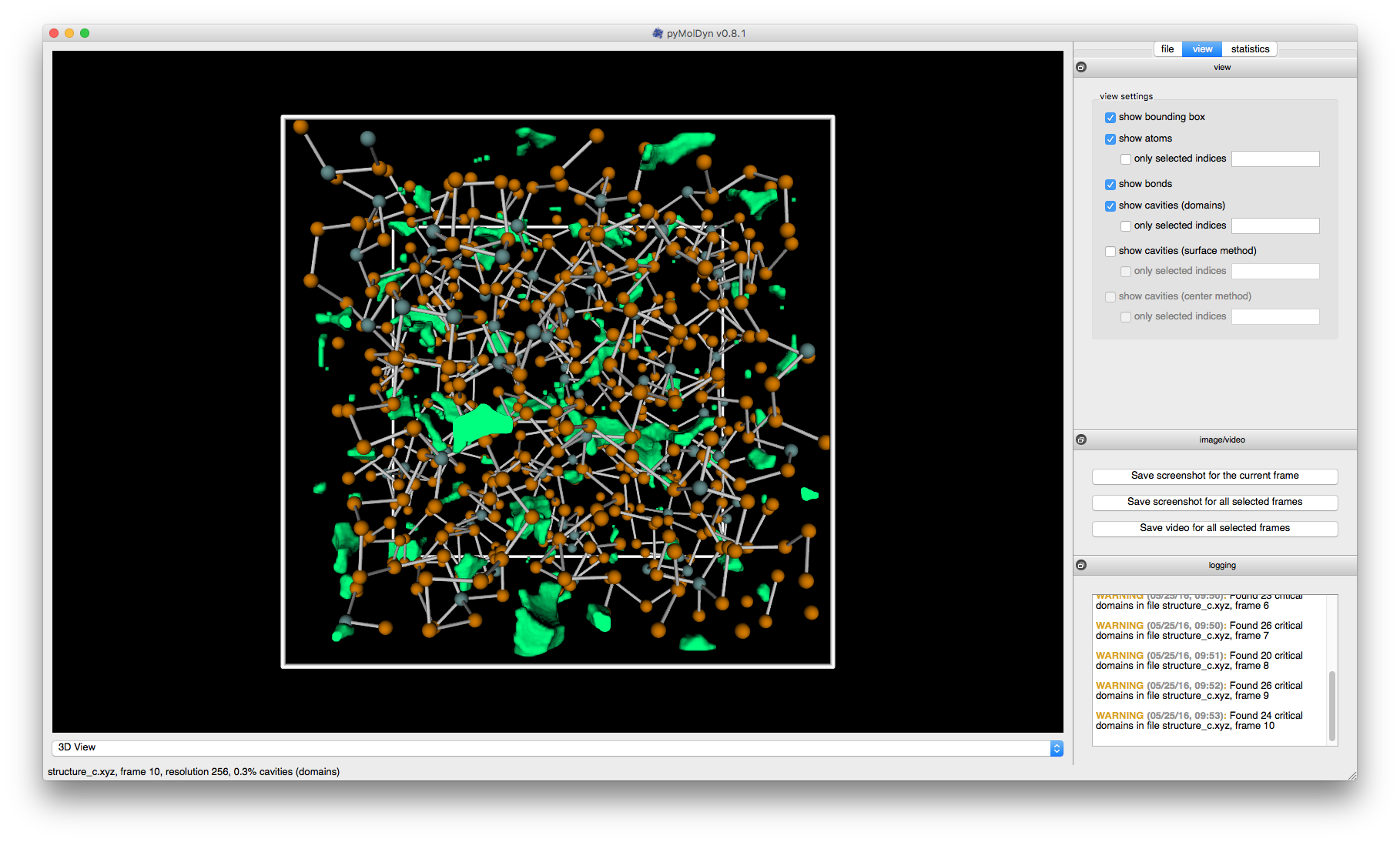
Atoms, bonds, cavities and the cell will then be shown in the (previously black) area on the left side of the window.
WARNING appears in the logging window if there are cavity domains consisting of a single cell of the discretization grid. The calculation should be repeated with a higher resolution to reduce the number of numerically unstable cavity domains.
Step 4: Adjusting the view
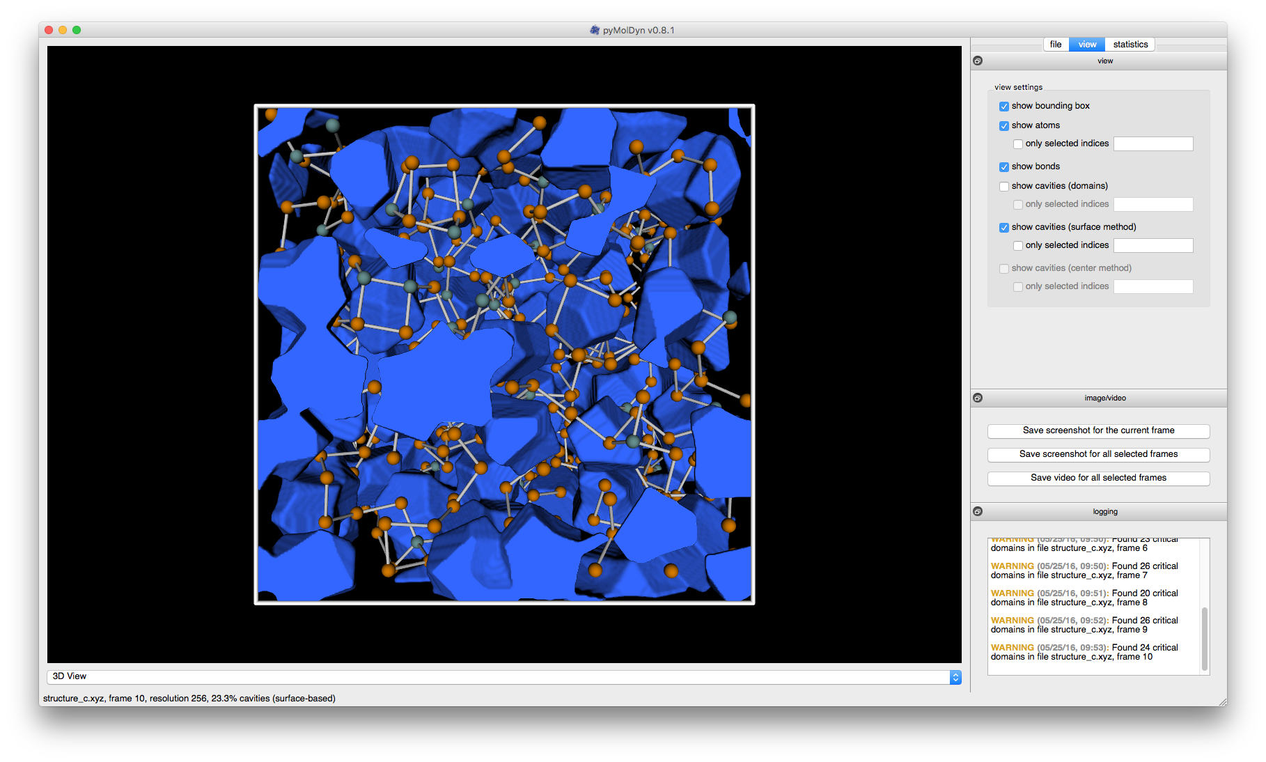
Checkboxes in the view tab control what is shown.
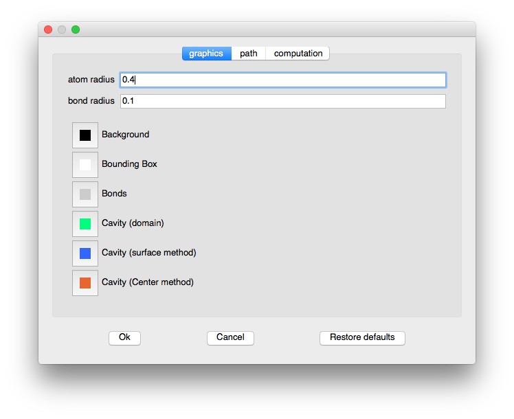
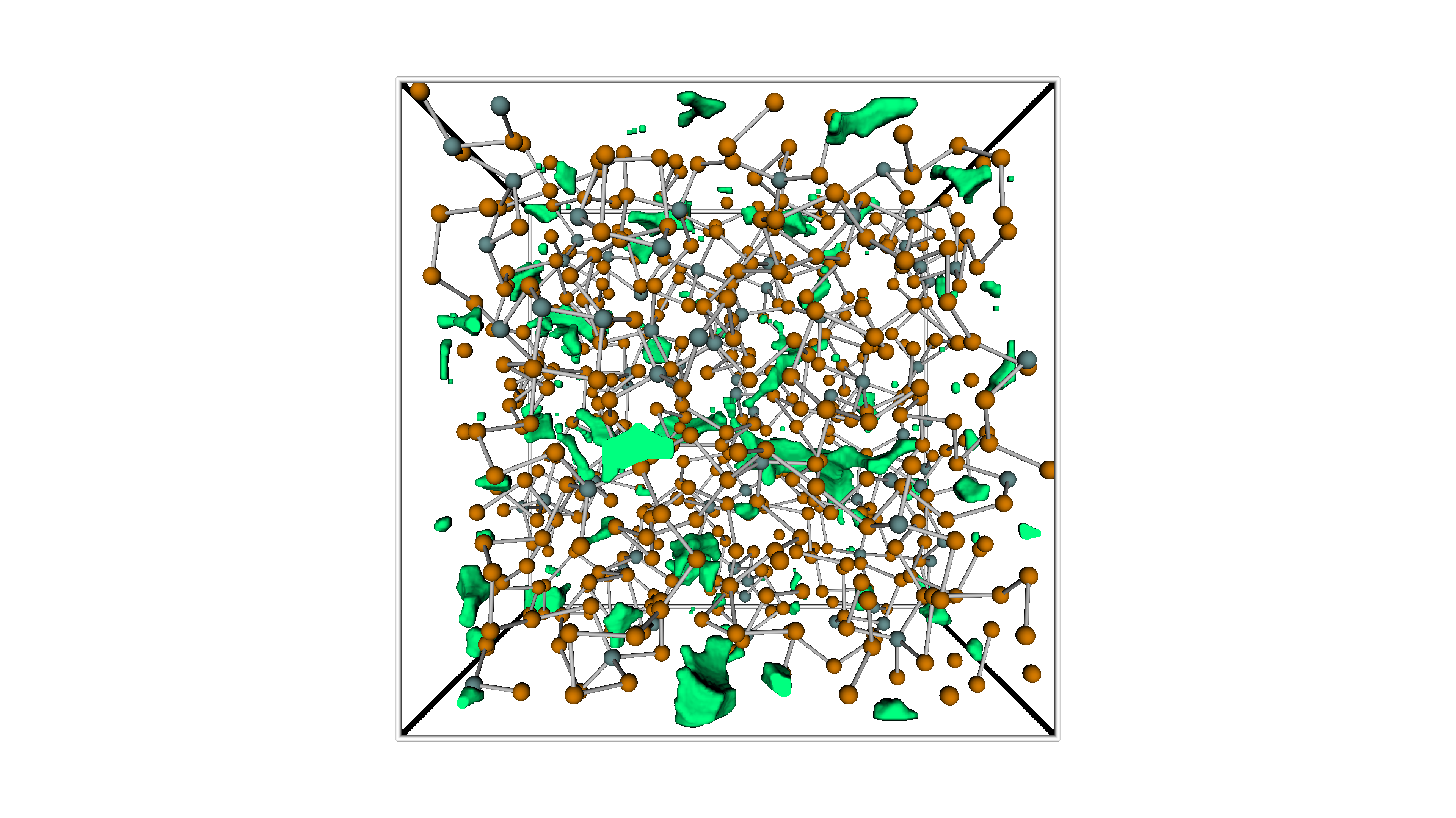
To adjust the colors of cavities, bonds, bounding box or background, open the preferences (in the menu click pyMolDyn → Preferences) and click on the button of the color you want to change. After adjusting these settings, e.g. by setting the background color to white, click on the Ok button for your changes to take effect.
To rotate the camera, click on the area on the left and move the mouse. For translation, press the alt key while doing this. You can zoom using the scroll wheel and to reset the view back to the default perspective, press the r key.
Next steps: Optional features
In this section, we describe additional features of pyMolDyn and how to use them.
Screenshots/video export
Once you are satisfied with the display of the atoms and cavities, you can export screenshots or videos by using the image/video panel at the bottom right of the window. Click on Save screenshot and select the location you want to save the screenshot to. Confirm this selection using Save and a high resolution screenshot will be created.
Pair Distribution Functions
Pair distribution functions can be calculated and visualized and the corresponding data output. Click on the dropdown menu at the bottom of the application window and select Pair Distribution. You can then select the elements (or cavities), the plot range, a smoothing kernel and its bandwidth (with 0.4 being the default). After clicking on Plot the RDF graph will be shown.
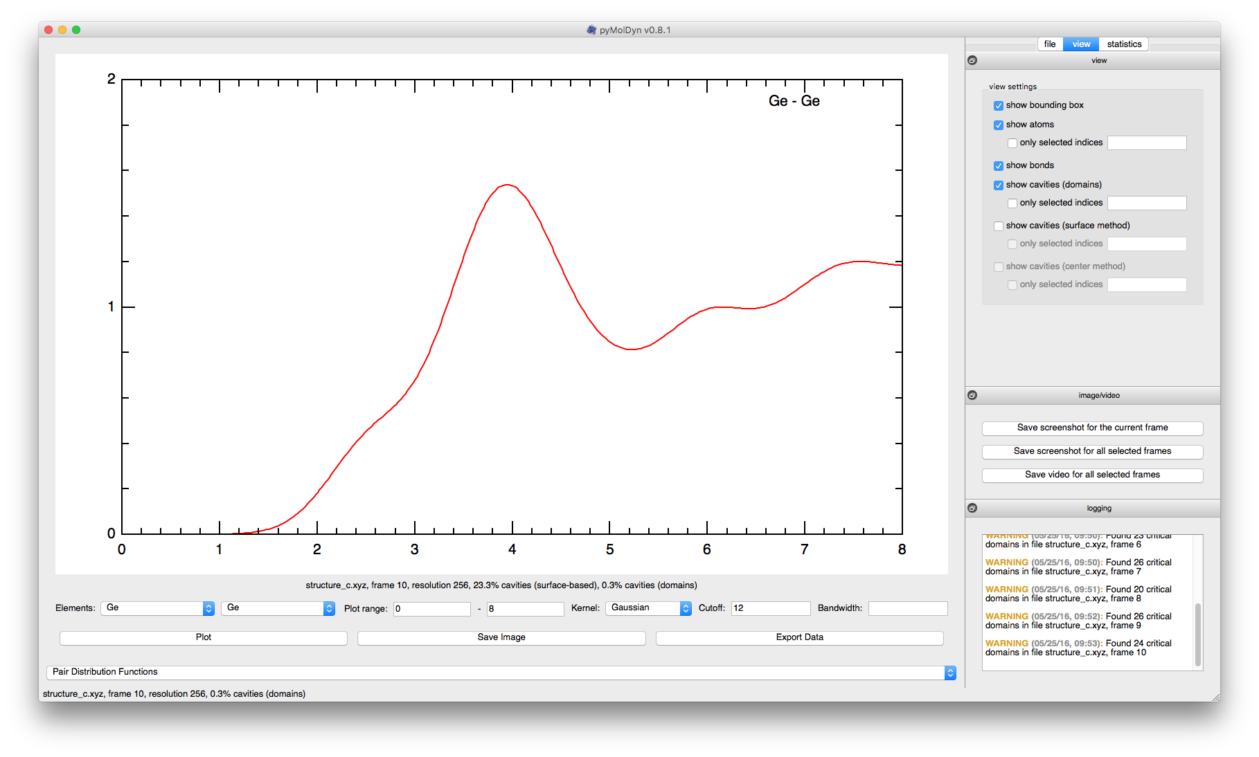
The default smoothing kernel is Gaussian, with the bandwidth parameter being used as sigma. For more information on the smoothing kernels, see the pyMolDyn Documentation. A bandwidth of 0 will prevent smoothing and show each data point as a peak of height 1. This can be useful, but visually overlapping peaks might be misleading.
Cavity Histograms
Histograms volume or surface area of cavity domains, surface-based and center-based cavities can be displayed and exported by pyMolDyn. Click on the dropdown menu at the bottom of the application window and select Cavity Histograms.
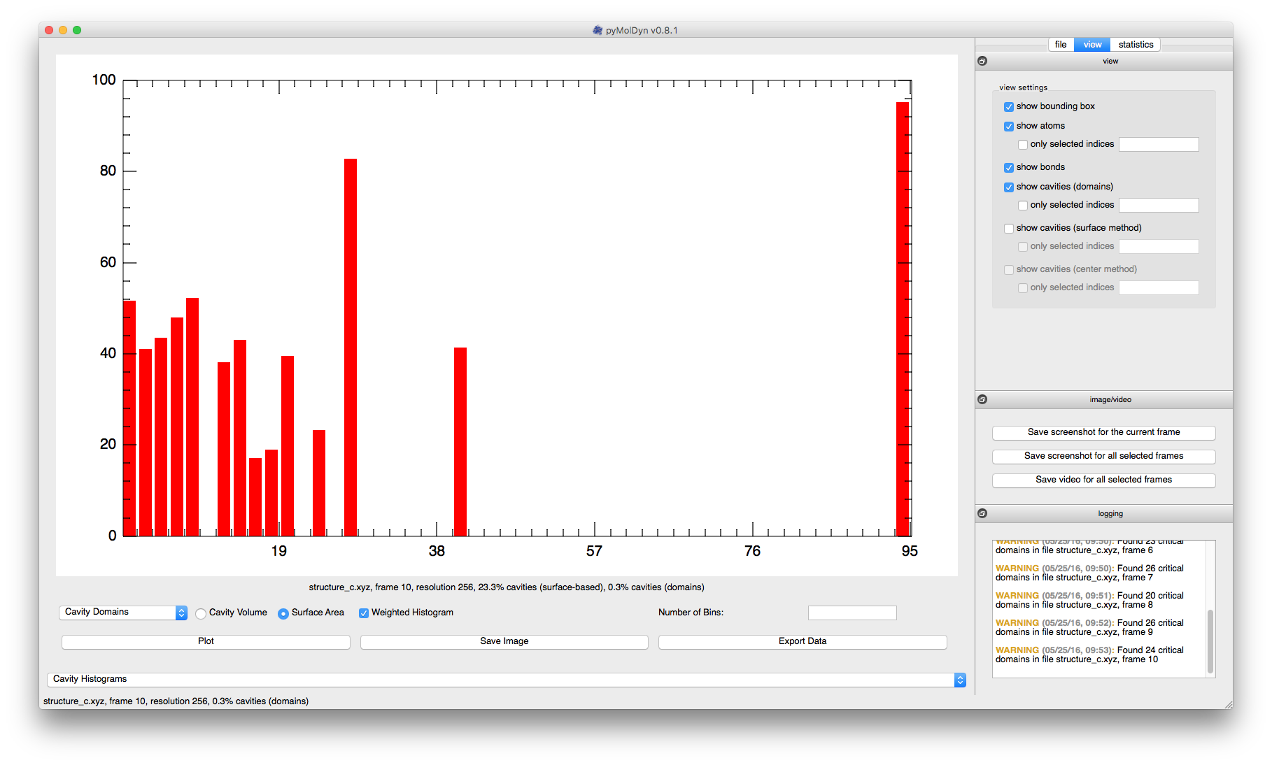
Select a cavity definition and whether cavity volume or surface area should be used, then click Plot. You can adjust the number of bins and whether the histogram should be weighted or not, and the histogram will be updated after another click on the Plot button. To save an image of the histogram or to export the data as text, click the corresponding buttons.